Statistics Refresher
An understanding of statistical concepts and methods can help you make informed decisions when assessing external scientific evidence. There are two main branches of statistics: (1) descriptive statistics and (2) inferential statistics.
Descriptive statistics summarize and describe important features of the data. They most often use numerical measures (means, standard deviations) or graphical measures (boxplots and scatter plots).
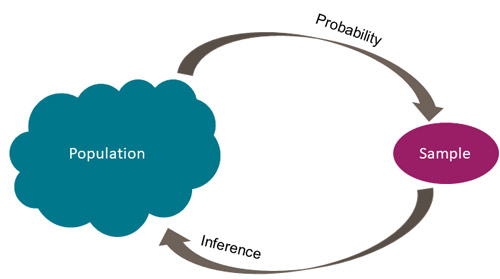
Inferential statistics generalize findings from a random sample to make inferences about a population (as illustrated in Figure 1). Researchers use inferential statistics to make quantitative conclusions about assessment and treatment approaches of interest based on hypothesis testing.
Figure 1. Inferential Statistics

You will encounter a variety of statistical tests, and the types of statistical measures used in a study depend on the type of data collected. This page addresses common statistical terms and their implications in audiology and speech-language pathology research literature:
- treatment literature
- statistical significance
- clinical significance (effect sizes)
- basic concepts in a meta-analysis
- statistical precision
- screening/diagnostic literature
Common Statistical Terms in Treatment Literature
Statistical Significance
Statistical significance is a common term used in research to assess the strength of a study’s results. To determine if an experiment is statistically significant or not, researchers use a calculated probability, called a p value, to try to reject a null hypothesis (i.e., that there is no difference between two groups). A p value is the probability that the observed data from the treatment group and the comparison group are, in fact, different from each other and that this difference was not due to chance.
A very small p value under the pre-determined cutoff threshold indicates a very low chance that the observed data would occur if the outcomes of both groups were actually the same. Therefore, the differences observed in the data are statistically significant because the researchers rejected the null hypothesis.
The cutoff threshold for statistical significance can vary in research. However, a common threshold is .05 (p≤ .05). P values greater than .05 (p> .05) reflect that the differences are not statistically significant.
P values are greatly influenced by the sample size of a study. For example, a study with a large sample size and a small effect size may be statistically significant, and a study with a small sample size and a large effect size may not meet statistical significance.
Quick tip:
Statistically significant findings do not necessarily mean clinical significance. Statistical significance relates only to the compatibility between observed data and what would be expected under the null hypothesis.
Clinical Significance
Clinical significance refers to the practical value or importance of the intervention effect. It means that the intervention makes a meaningful difference in the severity or functioning of the people with the disorder. In this respect, p values have their limitations because they do not tell us about the size of the effect or how well the intervention works. Therefore, researchers are beginning to encourage the use of additional measures to demonstrate a meaningful difference. Clinical significance demonstrates the size of the effect between two variables and, ultimately, the clinical importance of the relationship.
An effect size is a common measure of clinical significance used to estimate the differences between two groups (i.e., standardized mean difference) or the strength of an association between variables (e.g., odds ratio, relative risk ratio, Pearson’s coefficient). The following metrics are common indices used to calculate effect size.
Table 1. Diagnostic 2 x 2 Table
| Groups | People w/ disorder | People w/o disorder |
| Control | A | B |
| Experimental | C | D |
Table 2. Types of Effect Sizes
| Index | Description | Comments | |||||||
| Odds ratio (OR) |
The likelihood of an event occurring in one group (experimental) compared to the likelihood of the same even occurring in a different group (control). OR is defined as in Table 1.
|
|
|||||||
| Risk ratio (RR) |
The probability of an outcome occurring in one group (experimental) divided by the probability of an outcome occurring in another group (control). RR is defined as in Table 1.
|
||||||||
| Cohen's d | The difference of two group means divided by the population standard deviation. |
Cohen's d and Hedges' g effect sizes, sometimes called "standardized mean differences," are interpreted in the same way:
|
|||||||
| Hedges' g |
Hedges' g is similar to Cohen's d. The only difference is that Hedges' g uses the pooled standard deviations of all experimental groups and the control group instead of the population standard deviation. Hedges' g is considered a conservative measure of the Cohen's d effect size. It is also known for more precise calculations for studies with smaller sample sizes. |
||||||||
| Pearson's coefficient (r) |
Pearson's r is a correlational coefficient—which demonstrates the association between two variables—that assumes the sample represents the population. The Pearson's r value, which can be positive or negative, merely measures the positive or negative association and doesn't indicate a direct causation. |
Pearson's r ranges from -1 to 1, and negative r values indicate a negative association (Ferguson, 2009).
|
Basic Concepts in Meta-Analysis
Forest Plots
Researchers use a statistical procedure known as a meta-analysis to combine data from studies addressing the same or similar questions and use forest plots to visually display the treatment effects.
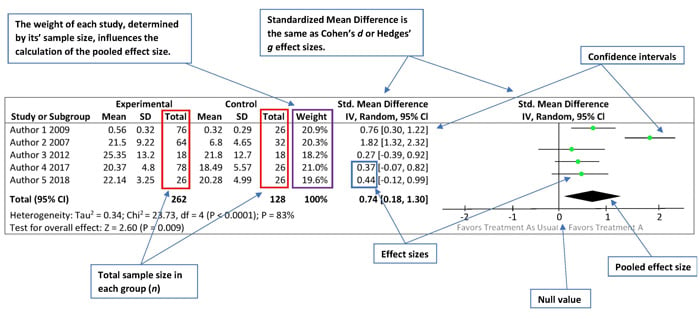
Figure 2 below is an example of a data chart and forest plot from a simulated meta-analysis examining the effects of the experimental group (the group that received the treatment) compared to the effects of the control group (the group that received no treatment or an alternative treatment) on expressive language outcomes.
Figure 2. Example of Data Chart and Forest Plot

On the Left Side
The left side of the forest plot is a data chart of all studies included in the meta-analysis and each study’s results comparing the relationship between the experimental group (Treatment A) and the control group (Treatment as Usual). The chart includes the total number of subjects in each group, the weight of each study (i.e., the influence of each study on the overall results), the effect size estimates and their respective confidence intervals, and the combined data from all studies.
On the Right Side
The right side of the forest plot reveals a graphic representation of the same information.
The various effect size estimates for each study are depicted as the green squares, with the size of each square representing the weight of the study within the meta-analysis. The black horizontal lines going through the green squares depict the confidence intervals. Longer lines represent wider confidence intervals and less reliable results (see Statistical Precision subsection below to learn more about confidence intervals).
The black solid line in the center of the forest plot represents the null value or what is also called the “line of no effect.” Individual study estimates going through the null value indicate that there may be no difference between the experimental and control groups. The distance between the green dot and the null value reflects the magnitude of the effect size. In other words, the farther away the green squares are from center black line, the larger the effect size.
The black diamond represents the pooled effect size—that is, the point estimate and confidence intervals when you combine all the data from the weighted studies.
Statistical Precision
Because results are always subject to some degree of error, the exact value is never truly known. Instead, the results are provided as estimates, and you need to determine how precise the estimates are in relation to the statistics’ true value. In Figure 3, black lines on each side of the green boxes reflect the precision of each effect size. The following factors can measure precision:
- Confidence interval (CI) is a range of values in which the true value most likely lies. Cl is always calculated with a specified confidence level, typically using 95% or 99% confidence level. This means that if the same tests are performed multiple times and the confidence level is 95%, the CI will contain the true value 95% of the time.
- Smaller sample sizes are likely to have wider CIs. This affects the precision of the findings. Studies with larger sample sizes would have more precise findings.
- Standard deviation estimates the variability or spread within a sample population and tells you how far out the data are from the mean or average. You frequently see standard deviation on the normal distribution of the bell-shaped curve. In a normal distribution, 95% of the sample data will fall within 2 standard deviations of the mean.
- Standard error of the mean is the standard deviation of the mean’s sample distribution (how close the sample means are to the population’s “true mean”).
- Researchers usually use standard error of measurement (SEM; Musselwhite & Wesolowski, 2018) when analyzing a diagnostic tool’s test reliability. SEM, which is calculated using repeated measures, estimates how different a test-taker’s observed score is from the “true score.”
Common Statistical Terms in Screening/Diagnostic Literature
Statistics in diagnostic research are used to evaluate the accuracy of assessment or screening instruments and their ability to accurately predict the presence or absence of a condition or disease. Several statistical terms used in treatment literature can also be found in screening or diagnostic research. For example, OR and relative risk are common measures that researchers use to estimate the effect size of dichotomous outcomes (e.g., yes/no). In audiology and speech-language pathology literature, researchers typically use OR and relative risk to measure the effectiveness of a test in order to identify individuals with the disorder versus individuals without the disorder.
Validity and Reliability
When reading research, it is important to consider the reliability and validity of screening or diagnostic assessment tools. These concepts are essential to determining the accuracy of any diagnostic assessment.
Reliability measures the extent to which the diagnostic tool produces stable and consistent results. There are two general types of reliability: interrater reliability and intrarater reliability.
Interrater reliability refers to the likelihood that different raters rating the same or comparable participants would give the same rating. Intrarater reliability, sometimes referred to as “test–retest reliability,” refers to the likelihood that the same rater would again give the same rating to the same patient on the same or subsequent exam, assuming that nothing about the patient’s status had changed.
Validity tells you whether an assessment is measuring what it is intended to measure. Reliability is a necessary property of any valid assessment, but it is not enough to guarantee the validity of the assessment. So, an assessment could be reliable.
Figure 3. Representations of High and Low Reliability and Validity

Diagnostic Accuracy
Diagnostic accuracy is the ability of the test to discriminate people with the disorder from people without the disorder. Different aspects of diagnostic accuracy can be quantified by statistical measures such as sensitivity and specificity, predictive values, and likelihood ratios. These measures are very sensitive to the characteristics of the population in which they are measured.
Sensitivity and Specificity
Sensitivity and specificity can be used to discriminate people with and without the disorder. Sensitivity, computed as a percentage, represents the probability of getting positive test results in people with the disorder. It is the proportion of the individuals who are screened positive with the disorder among the total group of people with the disorder. Specificity is a measure of diagnostic accuracy that is complementary to sensitivity. Specificity, also computed as a percentage, represents the probability of getting negative test results among the people without the disorder. It is the proportion of the individuals who are screened negative with the disorder among the total group of people without the disorder.
Example
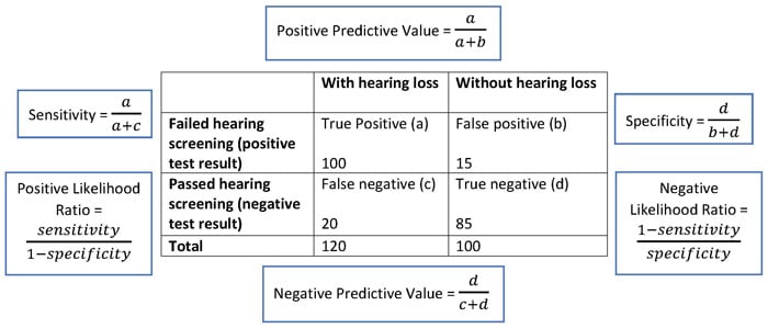
Figure 4 represents an example of a 2 × 2 diagnostic table of hearing screening results, with equations. Based on the equations, the sensitivity of the hearing screening is 83%, which means that 83% of the people who fail the hearing screening are diagnosed with a hearing loss after a full audiological examination. A specificity of 85% demonstrates that the hearing screening can rule out hearing loss in 85% of the people without hearing loss.
Figure 4. Example 2 x 2 Diagnostic Table of Hearing Screening Results (With Equations)

Predictive Value
Predictive value is another measure for diagnostic accuracy. This measure gives insight to the observed results and the chances that they are the true results.
- Positive predictive value (PPV) is the probability of having the disorder among the individuals with positive screening results.
- Negative predictive value (NPV) is the probability of not having the disorder among the individuals with negative screening results.
Both PPV and NPV are sensitive to the prevalence of the disorder among the examined people. When the prevalence of the disorder increases in a population, PPV increases, whereas NPV decreases.
Example
In Figure 4, the positive predictive value of the hearing screening is 87%, and the negative predictive value of the hearing screening is 81%. When a hearing screening yields a positive result for hearing loss, the patient has an 87% chance that they truly have a hearing loss.
Likelihood Ratio
Likelihood ratio is the probability of a given diagnostic test score would be expected in an individual with the disorder of interest compared to the probability that the same result would be expected in an individual without that disorder. The calculations for positive and negative likelihood ratios consider the sensitivity and specificity of the test, which makes likelihood ratios less susceptible to the influence of a disorder’s prevalence rate.
Likelihood ratio for positive test results (LR+):
“LR+ reflects confidence that a positive (disordered or affected) score on a test came from a person who has the disorder rather than from a person who does not.” (Dollaghan, 2007, p. 93)
- LR+ represents the ratio of the probability that a positive test result occurs among the people with the disorder to the probability that a positive test result occurs among the people without the disorder. LR+ is usually higher than 1 because the people with the disorder tend to have higher positive test results. LR+ is the best indicator for ruling in a diagnosis.
Likelihood ratio for negative test results (LR–):
“LR– concerns confidence that a score in the unaffected ranges come from a person who truly does not have the target disorder.” (Dollaghan, 2007, p. 93)
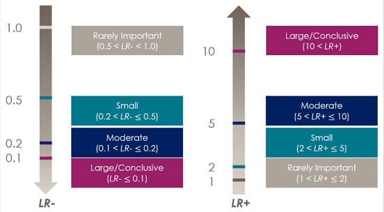
- LR– represents the ratio of the probability that a negative test result occurs among the people with the disorder to the probability that a negative test result occurs among the people without the disorder. Thus, LR– reflects how much less likely the negative test result will occur among the people with the disorder than among the people without the disorder. LR– is usually less than 1 because the people without the disorder will have a higher rate of negative test results. Higher LR+ indicates greater confidence that a positive screening result is truly from a person with the disorder. Lower LR– indicates greater confidence that a negative screening result is truly from a person without the disorder. An LR+/LR– of 1.0 is neutral, indicating an equal chance that a test score could come from a person with or without the disorder, which suggests that the clinician may need to choose another screening or diagnostic tool with better diagnostic accuracy. Figure 5 shows one of the many examples of how to interpret likelihood ratios (Jaeschke, Guyatt, & Lijmer, 2002).
Figure 5. Representation of Negative Likelihood Ration (LR-) and Positive Likelihood Ration (LR+)

In Figure 5, LR+ equals 5.53, which means that you can be moderately confident that a failed hearing screening comes from a person with hearing loss. LR– is also equal to 0.2, which means that you can be confident that an unremarkable hearing screening probably (with moderate likelihood) came from a person without hearing loss.
References
Dollaghan, C. A. (2007). The handbook for evidence-based practice in communication disorders. Baltimore, MD: Brookes.
Ferguson, C. J. (2009). An effect size primer: A guide for clinicians and researchers. Professional Psychology: Research and Practice, 40(5), 532–538. https://doi.org/10.1037/a0015808
Jaeschke, R., Guyatt, G., & Lijmer, J. (2002). Diagnostic tests. In G. Guyatt & D. Rennie (Eds.), Users' guides to the medical literature: Essentials of evidence-based clinical practice (pp. 187–217). Chicago, IL: American Medical Association.
Musselwhite, D. J., & Wesolowski, B. C. (2018). Standard error of measurement. In B. B. Frey (Ed.), The SAGE encyclopedia of educational research, measurement, and evaluation (Vol. 4, pp. 1587–1590). Thousand Oaks: SAGE.


